The difference between training data distribution and the production data distribution is an undeniable reality within the AI field.
Recently With the development of Deep Learning Techniques and the Hardware capabilities the challenge is not longer how to map the inputs to predict the outputs, BUT how to know when you don’t know the output. how to tell that your model isn’t confident from it’s prediction.
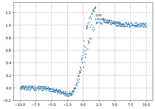
Let's delve into an example to clarify things further. Imagine we're dealing with a regression problem, and our dataset resembles the one depicted in Figure 1.
figure 1
How should we approach this dataset? If we opt for a neural network with just one output neuron to model this data, what do we do with the Y values when X falls within the range [0 to 2], for instance?
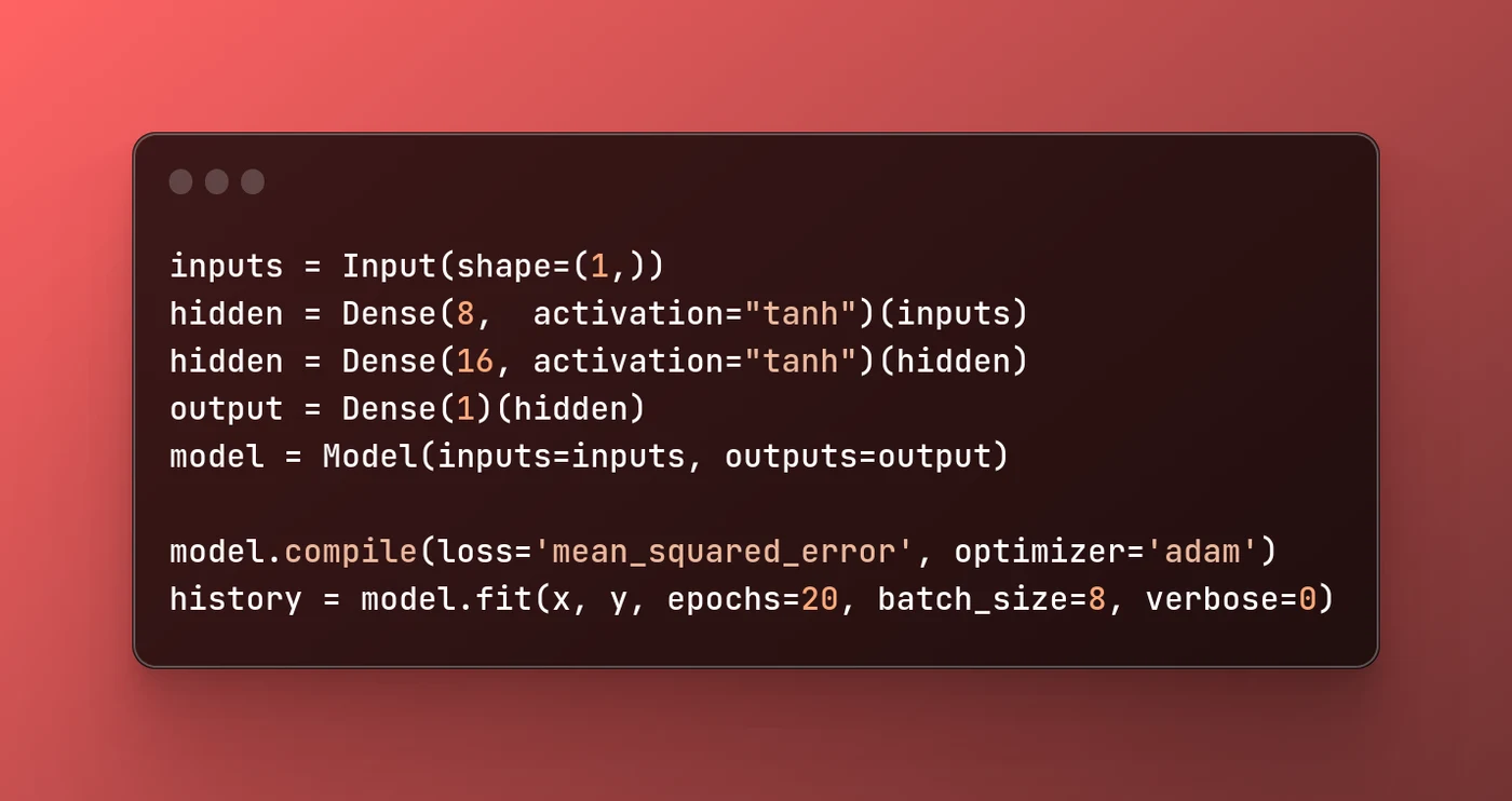
Now, let's explore how we might address this using a standard neural network. The following code is used to train a neural network comprising two hidden layers with tanh activation function and one neuron in the output layer.
Note: “You need to install tensorflow & tensorflow_probability”
As is evident from our approach, we have specifically chosen the mean squared error (MSE) as our loss function. MSE is a commonly used loss function in regression tasks, aiming to minimize the squared differences between predicted values and ground truth labels.
In addition, we've selected the Adam optimizer for training our model. Adam is a popular optimization algorithm known for its efficiency and adaptability. It combines techniques like momentum and adaptive learning rates to help models converge faster and perform well on a wide range of tasks.
These choices were made to optimize the training process and enhance the model's ability to capture patterns within the data effectively.
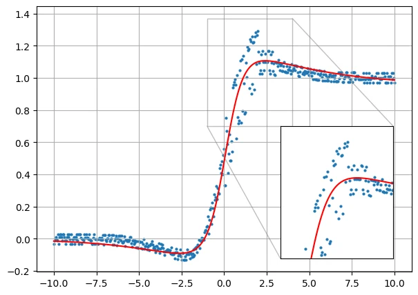
By employing the code mentioned earlier, we trained the neural network on the dataset illustrated in Figure 1. Now, let's examine the model's predictions.
figure 2
As the visual representation in Figure 2 demonstrates, the model's predictions align closely with the dataset, exhibiting minimal errors. This alignment reflects the model's competence in capturing and reproducing the underlying patterns in the data.
However, the situation becomes more intriguing when we shift our focus to the data range where X values fall between 0 and 2. Within this specific interval, it becomes essential to explore the model's behavior in greater depth. Here, we confront a critical challenge: how do we determine the degree of certainty or uncertainty in our model's predictions? Or in a statistical term how to calculate the "variance". As High variance signifies that the data points are dispersed over a wide range, indicating uncertainty.
Fortuitously, the concept of probabilistic models has emerged as a solution to address this challenge. The fundamental distinctions between a conventional model and a probabilistic model can be summarized as follows:
In probabilistic models, our objective is not to predict a single deterministic output. Instead, we aim to predict a complete probability distribution, typically represented by well-known distributions like the Normal Distribution.
Probabilistic models are trained with a focus on minimizing the Negative Log Likelihood (NLL) between the observed data and the predicted probability distribution.
Note: “The Negative Log Likelihood (NLL) is a mathematical measure used in statistics and machine learning to assess how well a model's predictions align with actual observed data. It quantifies the disparity between the model's predicted outcomes and the real-world data. In essence, the lower the NLL, the better the model fits the data, as it indicates a closer match between predictions and reality. Minimizing the NLL during model training aims to enhance the model's accuracy and its ability to capture the underlying patterns in the data.”
Let's embark on a journey through a probabilistic model to explore these key differences. First, we'll construct a model with two significant modifications:
We will adopt the Normal distribution as the chosen prediction distribution. Consequently, the model's predictions will adhere to a Normal distribution characterized by specific mean and standard deviation.
Furthermore, we will adjust the structure of the final layer in comparison to the previous model. The updated design will encompass two neurons: one responsible for defining the distribution's Loc parameter, and the other for specifying the Scale parameter. This dynamic shift empowers the model to capture the inherent uncertainty within the data, an essential aspect in probabilistic modeling.
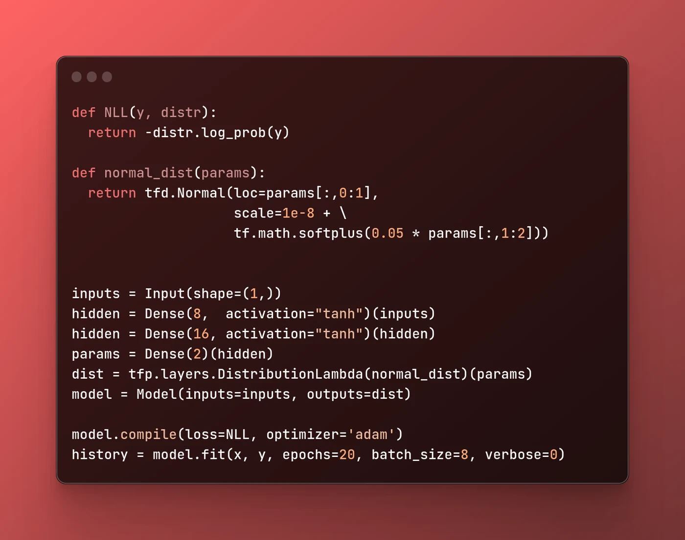
Indeed, we've initiated the changes as described, introducing two pivotal functions to enhance our probabilistic model's capabilities. Let's delve into the specifics of these modifications:
NLL Function:
The first function, aptly named "NLL" plays a fundamental role in our probabilistic model. It's designed to calculate the Negative Log Likelihood (NLL) of the probability distribution concerning the observed data and the actual ground truth.
In essence, it quantifies the alignment between the predictions of our model and the true data, shedding light on how well our model captures the underlying data distribution.
Normal Distribution Function (normal_dist):
The second function, "normal_dist" is equally crucial. It accepts a parameter argument, which is essentially an array with two values. These two values play pivotal roles in defining a Normal distribution:
params[0] signifies the "loc" which is the mean of the distribution, capable of taking both positive and negative values. It represents the center point around which the distribution is centered.
params[1] corresponds to the "scale" which is a critical parameter that determines the spread or standard deviation of the Normal distribution. Notably, it must be non-negative to ensure a valid distribution.
To handle this constraint and guarantee a valid scale, we employ the softplus function. This function not only ensures non-negativity but also mitigates extreme values, resulting in a more stable scale. Additionally, we include an epsilon value (1e-8) to prevent division by zero, a common safeguard in numerical computations.
These intricacies illustrate our model's adaptability and precision in modeling data distributions, especially when dealing with real-world data that often exhibits complex and nuanced characteristics.
Following the execution of the preceding code, the next step involves visualizing the model's predictions on the same dataset. This visual assessment will enable us to gauge whether the model's performance has improved, facilitating more informed decision-making.
figure 3
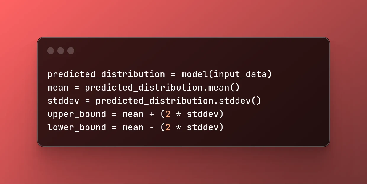
Note: You can simply get the mean and stddev of the model using the following code
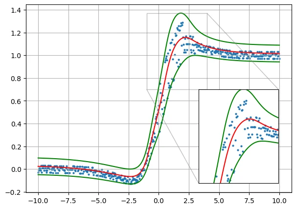
As depicted in Figure 3, the visual representation of our data reveals distinct characteristics regarding the mean (in red) and the standard deviation (stddev, in green). This visual analysis yields valuable insights into our probabilistic model's behavior:
Their interaction manifests differently across the spectrum of X values. Notably, when X resides within the interval [-2, 0], the distribution is notably compact, often described as "tight." Conversely, in the range [1, 2], the distribution noticeably widens, resembling a "spread."
This variance in distribution width serves as a natural confidence indicator. When the distribution is tight, precisely within the domain of [-2, 0], it signifies a robust level of confidence in our model's predictions. This suggests that the model's outputs are predictable and consistent in this realm.
In contrast, the widening distribution, most evident in the [1, 2] range, represents a lower level of confidence. The broadening dispersion of data points reflects a higher degree of unpredictability, underlining the model's decreased certainty in this specific region.
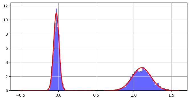
Now, we'll conduct a more detailed examination of specific data slices, precisely when X assumes the values of -1.5 and 1.5.
figure 4
In the subsequent figure, we delve into the Probability Density Function (PDF) for these particular X values. On the right-hand side of the figure, you'll find the PDF associated with X = -1.5, while on the left, we present the PDF corresponding to X = 1.5. This scrutiny allows us to gain a finer-grained perspective on the distribution of probabilities and outcomes associated with these specific data points.
What we have unveiled in this context is a concept known as Aleatoric Uncertainty. This form of uncertainty is intricately linked to the inherent variability present within the data or system under consideration. It's an uncertainty that cannot be eliminated or reduced through enhanced modeling or increased data volume. Rather, it represents the fundamental and irreducible variability within the data or system, and understanding it is pivotal for making informed decisions in scenarios where such variability plays a critical role.
Conclusion:
As demonstrated through a regression problem and the evolution of our modeling approach, probabilistic models offer a promising solution. These models deviate from the traditional deterministic output framework, instead focusing on predicting complete probability distributions, often leveraging the Normal Distribution.
Training probabilistic models involves minimizing the Negative Log Likelihood (NLL), emphasizing a better fit to the data. The critical insight gained from these models is the ability to quantify and understand the inherent uncertainty in predictions. The balance between a tight distribution, signifying high confidence, and a wide distribution, indicative of lower confidence, enables us to navigate scenarios with varying degrees of certainty.
Moreover, specific data slices and Probability Density Functions (PDFs) provide a granular view of the model's behavior and its implications in decision-making. The concept of Aleatoric Uncertainty, rooted in the irreducible variability within data or systems, serves as a pivotal consideration.
In essence, this exploration underscores the significance of probabilistic modeling and the essential role it plays in addressing the challenges posed by data distribution differences. By acknowledging and managing Aleatoric Uncertainty, AI practitioners can make more informed decisions in real-world applications, where uncertainty is an ever-present reality.